

Envelope analysis: finding a bearing fault the ordinary spectrum cannot show
A failing bearing can look quiet in the FFT. Four steps bring the fault out, and one of them decides whether it works.
The puzzle
A bearing is failing, but the ordinary spectrum shows nothing. Each time a rolling element hits a defect on the outer race it makes a tiny impact. That impact excites a high-frequency resonance in the structure, which rings for a moment and dies out. In the raw signal the ringing is buried under shaft harmonics and noise.
Why the FFT misses it
The energy of each impact is spread over a wide band far above the fault frequency. The FFT of the raw signal shows the carrier, which is the resonance, but not the repetition rate of the impacts, which is the fault.
The four steps
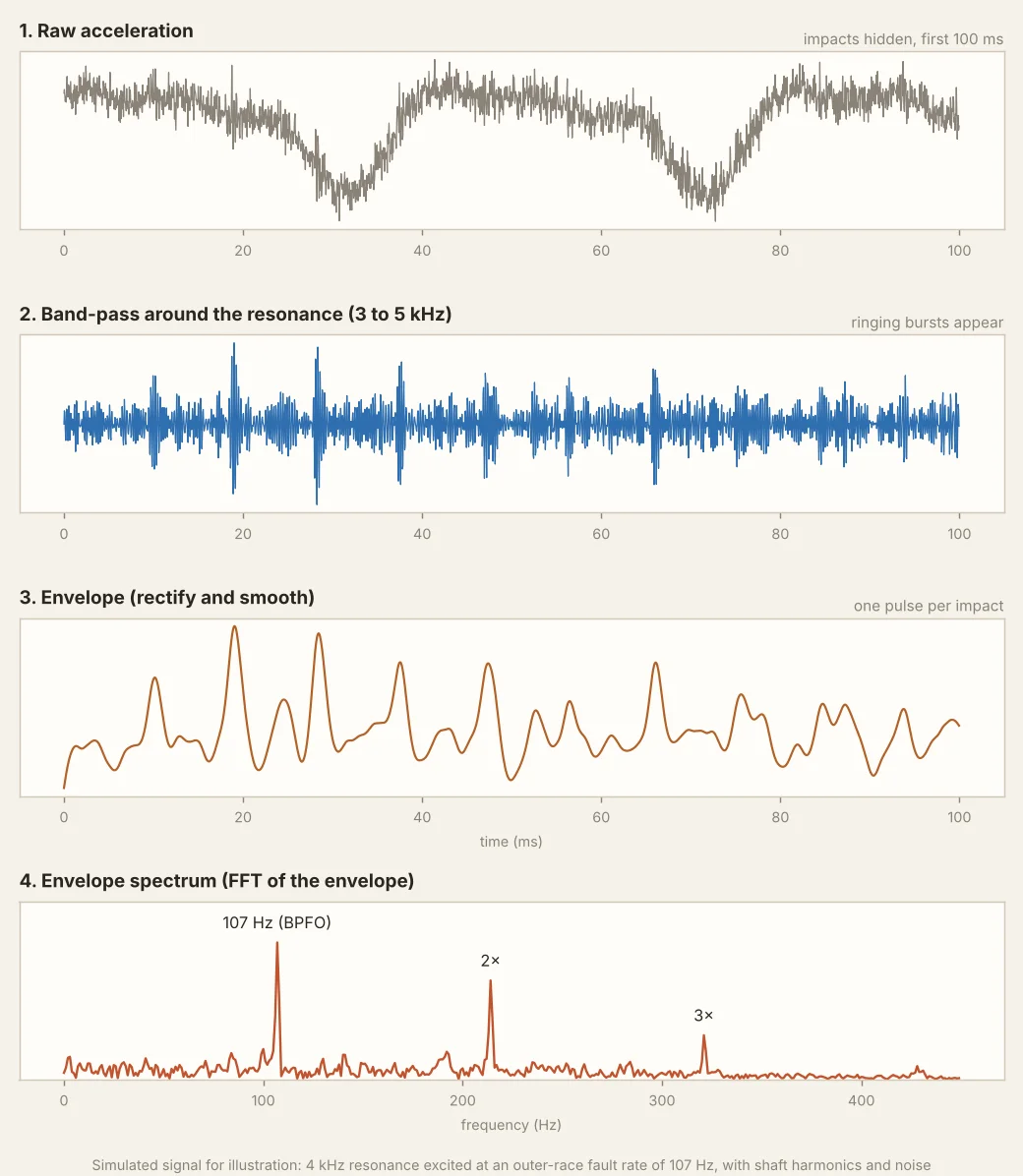
- Start with the raw acceleration signal. The faults are invisible.
- Band-pass filter around the resonance (about 4 kHz in the example). The ringing bursts appear.
- Rectify and smooth to get the envelope, which has one pulse per impact.
- Take the FFT of the envelope. Peaks appear at the fault frequency and its harmonics: here 107 Hz (BPFO) and 2× and 3× that.
Carrier and modulation
The raw signal is amplitude-modulated by the fault rate. The FFT of the raw signal shows the carrier (the resonance). The FFT of the envelope shows the modulation (the fault).
The hard part: choosing the band
The band you choose decides whether the fault is visible at all. A band below the resonance shows nothing, and a band that is too wide fills with noise. That is why tools such as the kurtogram exist: they search many bands and highlight the one where the signal is most impulsive.
Ways to pick the band
| Method | How it works | Watch out for |
|---|---|---|
| Kurtogram or spectral kurtosis | Scans bands and picks the one with the most impulsive content | Can pick a band dominated by a different impact source, such as a gear |
| Impact (bump) test | Tap the housing and read the natural frequency | Gives the structure, not the bearing, and changes with mounting |
| Fixed band by experience | Use the same band on every machine of one type | Needs checking when the mounting or sensor changes |
| Several bands | Run envelope in two or three bands and compare | Takes more time, but gives more confidence |
Reading the peaks
| What you see | Likely meaning |
|---|---|
| Peaks at the outer-race frequency and multiples | Outer-race defect. The load zone is fixed, so the peaks are steady. |
| Inner-race frequency with sidebands at shaft speed | Inner-race defect. The defect moves in and out of the load zone each turn. |
| Ball or roller spin frequency, often at twice that | Rolling element defect |
| Cage frequency, below shaft speed | Cage damage, or a bearing that is loose or sliding |
| Many multiples with a high floor | Late-stage damage. The signal is no longer a clean line series. |
When it struggles
- Very low speeds, where each impact is rare and the signal needs a long sample.
- Machines with strong gear mesh or other impacts in the same band.
- Noisy sensors, loose mounting or a poorly chosen sample rate.
Question to ask
On a real machine, what is the hardest part: picking the band, or interpreting the peaks? For many analysts it is the first, because everything after it depends on it.